
Hey there, coding explorer! Ever heard of Jupyter Notebooks? No worries if you haven’t – we’re here to make it super simple for you. Imagine a magical notebook where you can write code, play with data, and make cool things happen. That’s Jupyter, and we’re about to show you how to make it your new coding Best Friend!
From installation to creating your first code cell, we’ll walk you through each step, ensuring that you not only grasp the fundamentals but also develop a solid foundation for future coding endeavors. We’ll explore the interactive features, markdown capabilities, and how Jupyter Notebooks seamlessly integrate with popular programming languages like Python, R, and Julia.
This blog is your go-to guide for making Jupyter Notebooks your new coding playground. So, grab your coding backpack, and let’s embark on this adventure together – making Jupyter Notebooks a piece of cake for beginners. Ready, set, code! 🚀
What’s Jupyter Notebook?

Jupyter Notebook is like your online playground for coding adventures. It’s a open-source tool that lets you create cool documents mixing live code, math equations, pictures, and stories. So, what can you do with it?
Well, lots! You can clean up messy data, play with numbers, make cool charts, and even teach a computer to learn things – that’s machine learning, by the way! Jupyter supports more than 40 different programming languages, and one of them is Python, a super popular one.
Just a heads up, to get Jupyter Notebook on your computer, you’ll need to have Python installed first.
Jupyter Notebook goes beyond Python
Jupyter Notebook isn’t just a coding platform; it’s a polyglot’s dream come true. This versatile environment seamlessly integrates with a diverse range of popular programming languages, including Python, R, and Julia, allowing you to switch between them effortlessly.
Imagine this: you’re analyzing data in Python and stumble upon a specific statistical task that R excels at. With Jupyter Notebook, a simple switch of kernels lets you leverage R’s strengths without interrupting your workflow. It’s like having multiple powerful tools at your fingertips, ready to be deployed for any task at hand.
This seamless integration empowers you to:
- Embrace language diversity: Explore different languages without syntax restrictions
- Leverage strengths: Utilize the unique capabilities of each language for maximum effectiveness.
- Combine forces: Mix and match languages within the same notebook for complex analyses.
This flexibility empowers you to tackle diverse challenges and achieve groundbreaking results.
Ready to dive in and discover what this coding wonder can do for you? Let’s go! 🚀
1.Installation
Install Python and Jupyter using the Anaconda Distribution, which includes Python, the Jupyter Notebook, and other commonly used packages for scientific computing and data science.
This step is well explained here: Environment Preparation for Python: Anaconda and Jupyter Notebook – Around Data Science
When you finich all the steps of installation, launch Jupyter Notebook:
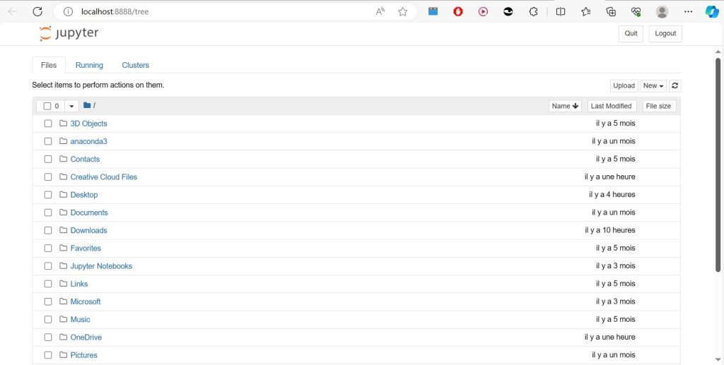
2.Creating a Notebook
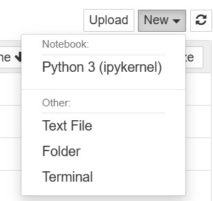
To create a new notebook, click on the new button at the top right corner. Click it to open a drop-down list and then if you’ll click on Python3, it will open a new notebook.
The web page should look like this:
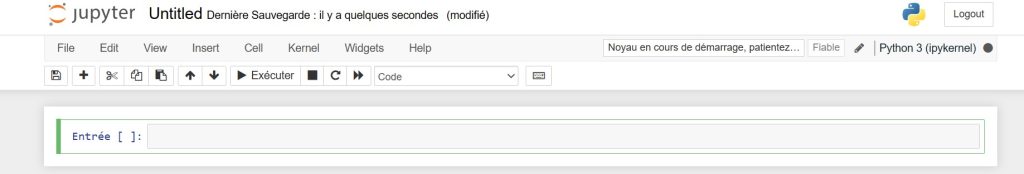
3.Renaming Your Jupyter Notebook
Jupyter Notebook, your gateway to data exploration and analysis, starts with a blank canvas aptly named “Untitled.” While this serves as a starting point, wouldn’t you want a name that reflects your project’s purpose and sparks curiosity? Renaming your notebook is a simple yet powerful step towards organization and clarity.
Say goodbye to the generic “Untitled” and embrace a more informative title. Simply click on the word itself, and a “Rename Notebook” dialogue box will appear. This is your chance to personalize your project!
Give your notebook a name that speaks volumes. Is it an analysis of the latest social media trends? Consider something like “Analyzing Twitter Sentiment on #ClimateChange.” Are you working on a machine learning model for fraud detection? “Building a Robust AI Model for Fraud Detection” would be a fitting title.

4.Crafting Your “Hello, World!” Program
- Access the Code Cell: Jupyter Notebook utilizes code cells to house your code snippets. To access a code cell, click on the ‘+’ icon located in the toolbar or press ‘Esc’ followed by ‘+’ (Insert Mode).
- Input the “Hello, World!” Code: Within the code cell, type the following code:
Python
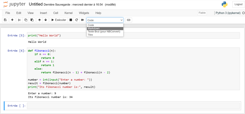
print("Hello, World!")- Execute the Code: To execute the code and witness its output, click on the ‘Run’ button located in the toolbar or press ‘Shift’ + ‘Enter’. Let’s see!

Note: When a cell has executed the label on the left i.e. ln[] changes to ln[1] (Entrée for me). If the cell is still under execution the label remains ln[*].
5.Building Cells of Jupyter Notebook
Jupyter Notebook, a powerful interactive computing environment, thrives on the concept of cells. These modular units serve as the foundation for code execution, text markup, and raw content. Understanding the different types of cells and their functionalities is essential for mastering Jupyter Notebook.
Types of Cells
1. Code Cells 💻:
Code cells are the heart of Jupyter Notebook, housing the code that drives computations and data analysis. The type of code accepted depends on the notebook’s language, such as Python or R. Executing code within a code cell generates output, displayed directly below the cell.
Example:
Python
def fibonacci(n):
    if n == 0:
        return 0
    elif n == 1:
        return 1
    else:
        return fibonacci(n - 1) + fibonacci(n - 2)

number = int(input("Enter a number: "))
result = fibonacci(number)
print("Its Fibonacci number is:", result)
- Output:

2. Markdown Cells 📝:
Markdown cells embrace the power of Markdown, a lightweight markup language, to create rich and engaging text content. These cells allow for formatting text, adding images, and embedding mathematical equations, enhancing the overall readability and presentation of your notebook.
Example:
Markdown
## The Fibonacci Sequence
The Fibonacci sequence is a series of numbers in which each number is the sum of the two preceding ones, starting from 0 and 1. Utilisez le code avec précaution. 
♦️Headers: Heading can be added by prefixing any line by single or multiple ‘#’ followed by space.
♦️ Lists: Easy Peasy. The list can be added by using ‘*’ sign. And the Nested list can be created by using indentation.
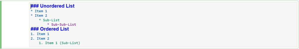
- Output:

♦️ Latex Equations ➕➖✖️➗: Latex expressions can be added by surrounding the latex code by ‘$’ and for writing the expressions in the middle, surrounds the latex code by ‘$$’.

- Output:

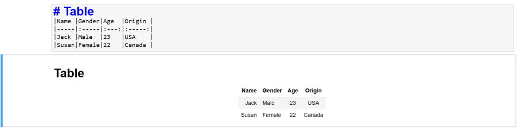
♦️ Table: A table can be added by writing the content in the following format.
♦️ The text can be made bold or italic by enclosing the text in ‘**’ and ‘*’ respectively.
3. Raw NBConverter Cells 💬:
Example:
This is a raw text cell. It will not be executed.
Raw NBConverter cells serve as repositories for raw text or code that is not intended for immediate execution. They are primarily used for storing notes, incorporating external content, or preserving code snippets that are not relevant to the current analysis.
6.Exploring the Capabilities of Kernels
Every Jupyter Notebook operates under the hood with a dedicated kernel, the driving force behind code execution and output generation. This unseen entity acts as a computational engine, processing your code within each cell and delivering the results for you to see.
Think of the kernel as a persistent entity dedicated to your entire document, not individual cells. This means that any modules imported in one cell remain accessible throughout the notebook. Imagine building a model – modules imported at the beginning are readily available for all subsequent analysis steps.
Here’s an example to illustrate this concept:
In[1]:
import pandas as pd

In[2]:
data = pd.read_csv("data.csv")
In this scenario, the pandas module imported in In[1] is available for use in In[2] and any subsequent cell within the same notebook.
Now, let’s explore the options available for managing kernels:
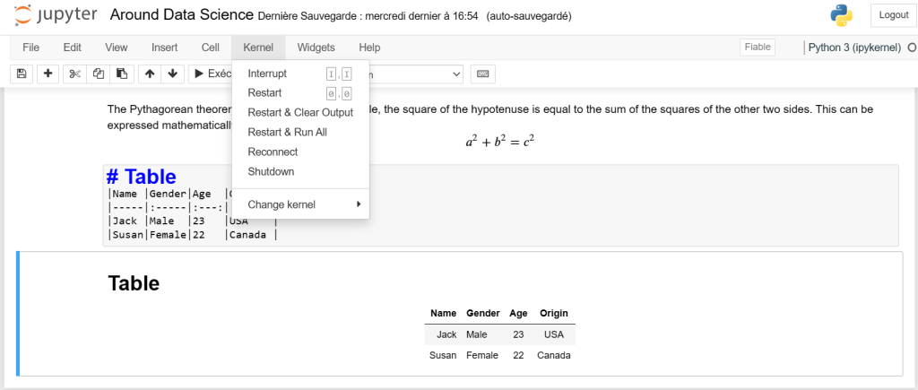
1. Restart: This action refreshes the kernel’s state, clearing all defined variables and imported modules.
2. Restart and Clear Output: This option performs a standard restart while also erasing any existing outputs displayed below the cells.
3. Restart and Run All: This powerful command combines restarting the kernel and automatically executing all cells within the notebook, top-down.
4. Interrupt: In the case of long-running programs or a stalled kernel, the interrupt option comes to the rescue. It forcefully terminates the current execution, allowing you to regain control and prevent unwanted delays.
🌟Mastering the kernel’s functionality empowers you to effectively manage your Jupyter Notebook environment, fostering a productive and efficient workflow for data exploration and analysis.
Welcome to a world where data reigns supreme, and together, we’ll unravel its intricate paths.


