
In the world of machine learning, especially in time series forecasting, prediction metrics play a crucial role in evaluating the performance of models. These metrics provide a quantitative way to measure the accuracy of a model’s predictions and help improve decision-making based on the results.
Without a robust evaluation strategy, relying solely on visual comparisons between actual and predicted values may lead to incorrect conclusions. In this guide, we will walk through the most important prediction metrics, break down their uses, and provide practical examples to help you grasp their significance.
Why Prediction Metrics are Essential in Machine Learning
Prediction metrics are important because they allow us to quantitatively assess how close a model’s predictions are to actual values. Whether it’s predicting future sales, stock prices, or customer behavior, these metrics help ensure that our model performs well and can generalize to unseen data.
In time series forecasting, the challenge is often greater because the data is sequential, and errors in one period can propagate into future predictions. For this reason, it’s critical to choose metrics that can accurately reflect model performance over time.
Explore : A/B Testing: A Data-Driven Approach to Boost Fast-Food Sales – Around Data Science
Key Prediction Metrics (With Practical Examples)
1. Root Mean Squared Error (RMSE)
Definition:
RMSE is a widely used metric that measures the square root of the average squared differences between predicted values and actual values. RMSE penalizes larger errors more than smaller ones, which is useful when you want to minimize big prediction mistakes.
Formula:
Where:
Example:
Imagine you are forecasting daily sales for a store over a week:
| Day | Actual Sales | Predicted Sales |
|---|---|---|
| 1 | 200 | 210 |
| 2 | 180 | 170 |
| 3 | 220 | 215 |
| 4 | 190 | 200 |
| 5 | 210 | 205 |
| 6 | 230 | 240 |
| 7 | 250 | 245 |
Using the formula, you can calculate RMSE for this forecast.
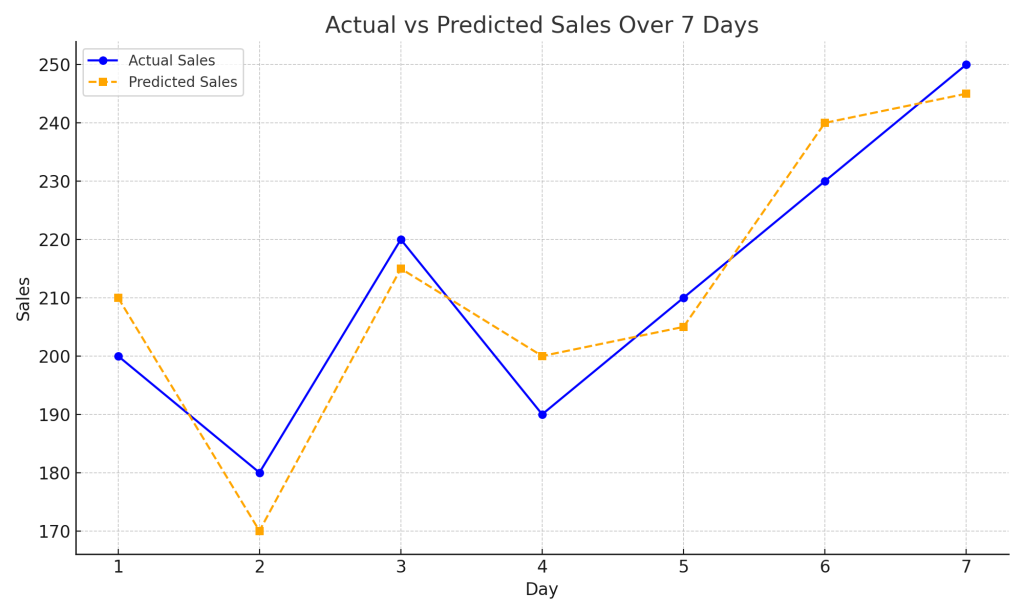
The errors are squared, averaged, and then the square root is taken. A lower RMSE indicates better model performance.
2. Mean Absolute Error (MAE)
Definition:
MAE measures the average magnitude of the errors in a set of predictions, without considering their direction. It provides an easy-to-understand metric as it simply calculates the absolute difference between predicted and actual values.
Formula:
Example:
Using the same sales data, MAE can be calculated by taking the absolute difference between each day’s actual and predicted sales, averaging the results. Unlike RMSE, it does not heavily penalize larger errors, which can make it a more balanced metric in certain cases.
3. Bias (Biais)
Definition:
Bias shows whether a model tends to systematically overestimate or underestimate the actual values. If the bias is positive, it means the model is underestimating; if negative, it is overestimating.
Formula:
Example:
Continuing with the sales example, if the bias is positive, the predicted sales are consistently lower than the actual sales. This is useful in identifying whether a model has a tendency to drift in one direction.
4. Congruence (Stability of Forecasts)
Definition:
Congruence, introduced by Kourentzes, measures how stable the predictions are across the entire forecast horizon. This metric is especially important in time series forecasting, where consistency across time is essential.
Example:
If you are forecasting sales for the next 12 months, congruence evaluates how much the model’s predictions fluctuate month-to-month. For instance, a high congruence means the forecast does not vary wildly between months, indicating a stable model.
5. Root Mean Squared Scaled Error (RMSSE)
Definition:
RMSSE is similar to RMSE but with one key difference: it scales the error by comparing it to a naïve baseline forecast. This is helpful when you need to compare different models or get a benchmark for model performance.
Formula:
Example:
Imagine you are forecasting next month’s sales based on last month’s data (a naïve forecast). RMSSE allows you to assess if your more complex machine learning model is actually better than this simple baseline.
Additional Useful Metrics in Time Series Forecasting
1. Mean Absolute Percentage Error (MAPE)
Definition:
MAPE measures the percentage error between actual and predicted values. It’s easy to interpret because it provides a percentage-based error, but it can be problematic with very small values.
Formula:
Example:
In forecasting scenarios where small values exist (e.g., predicting sales under 10 units), MAPE can lead to inflated errors. For instance, if you predict 5 units and the actual value is 1, MAPE might overemphasize the error.
2. Symmetric Mean Absolute Percentage Error (sMAPE)
Definition:
Formula:
Example:
If you are forecasting stock prices or demand,
3. Coefficient of Determination (R²)
Definition:
Formula:
Where
Example:
If your model has an R² of 0.85, it means that the model explains 85% of the variance in the actual data. A higher R² indicates a better model fit, but it should be used cautiously in time series contexts.
How to Choose the Right Metric for Your Model
When selecting prediction metrics for your machine learning model, consider the following:
- Data Type: Are you dealing with time series data or independent observations?
- Error Sensitivity: Do you want to penalize large errors more heavily? RMSE might be better than MAE in this case.
- Interpretability: If stakeholders need easily interpretable metrics, MAE or MAPE might be preferred.
It’s often a good idea to combine several metrics to get a comprehensive understanding of your model’s performance.
Ready to see a proof of concept? Check out this case study : House Prices Prediction using Linear Regression Model – Around Data Science
Conclusion
Prediction metrics are essential tools for assessing the accuracy of machine learning models, particularly in time series forecasting. By understanding the strengths and weaknesses of each metric, you can make informed decisions about which to use for your particular problem.
🌟For more in-depth guides and resources, explore Around Data Science hub. Dive deeper into specific topics, discover cutting-edge applications, and stay updated on the latest advancements in the field. Subscribe to our newsletter to receive regular updates and be among the first to know about exciting new resources, like our first upcoming free eBook on Artificial Intelligence for All! Don’t miss out!
Welcome to a world where data reigns supreme, and together, we’ll unravel its intricate paths


