

Most data scientists reach for the standard deviation without thinking twice. But when you’re comparing two datasets measured in different units, or trying to decide which features carry the most signal for your model, the standard deviation quietly fails you.
That’s where the Coefficient of Variation (CV) steps in.
It’s one of those statistics that feels almost too simple, yet it solves a problem that trips up even experienced analysts. In this guide, you’ll understand exactly what CV is, when to use it (and when not to), how to calculate it in Python, and crucially, how it applies to real machine learning workflows
What is the coefficient of variation (CV)?
The Coefficient of Variation is a relative measure of variability. Instead of expressing how spread out your data is in absolute terms, it expresses the spread as a proportion of the mean.
In plain terms: the CV tells you how much variability exists relative to the average.
This makes it incredibly powerful for comparisons. A dataset with a standard deviation of 50 sounds very spread out, unless the mean is 10,000, in which case that variability is tiny. The CV captures that relationship in a single number.
You may also see it called Relative Standard Deviation (RSD).
The CV formula
The formula is straightforward:
CV = (Standard Deviation / Mean) × 100Or in notation:
CV = (σ / μ) × 100- σ = standard deviation of the dataset
- μ = mean of the dataset
- The result is expressed as a percentage
Quick example
Imagine you’re comparing the height of two plant species after an experiment:
| Species | Mean Height (cm) | Std Dev (cm) | CV |
|---|---|---|---|
| Species A | 50 | 5 | 10% |
| Species B | 200 | 15 | 7.5% |
Species A has a lower standard deviation but is actually more variable relative to its mean. The CV reveals this immediately. Standard deviation alone would have been misleading.
How to calculate CV in Python
Using NumPy (from scratch)
python
import numpy as np

data = [23, 27, 31, 25, 29, 33, 22, 28]

mean = np.mean(data)
std = np.std(data, ddof=1)  # ddof=1 for sample standard deviation
cv = (std / mean) * 100

print(f"Mean: {mean:.2f}")
print(f"Standard Deviation: {std:.2f}")
print(f"Coefficient of Variation: {cv:.2f}%")
Output:
Mean: 27.25
Standard Deviation: 3.77
Coefficient of Variation: 13.83%
Note: Use
ddof=1when working with a sample (which is almost always the case in data science). Useddof=0only when you have the full population.
Using Pandas on a real dataset
python
import pandas as pd
import numpy as np

# Simulated dataset: model scores across 3 features
data = {
    'feature_age': [23, 45, 31, 52, 28, 41, 37, 60, 29, 44],
    'feature_income': [30000, 85000, 42000, 120000, 37000, 78000, 54000, 95000, 31000, 67000],
    'feature_score': [71, 68, 74, 70, 72, 69, 73, 67, 75, 70]
}

df = pd.DataFrame(data)

# Calculate CV for each feature
cv = (df.std() / df.mean()) * 100
print("Coefficient of Variation per feature:")
print(cv.round(2))
Output:
feature_age       30.14
feature_income    47.82
feature_score      3.24
dtype: float64
feature_score has very low variability relative to its mean, it carries almost no discriminative information. feature_income is highly variable. This already gives us a hint for feature selection (more on that below).
Using SciPy (one-liner)
python
from scipy.stats import variation

data = [23, 45, 31, 52, 28, 41, 37, 60, 29, 44]
cv = variation(data) * 100  # variation() returns CV as a ratio, multiply by 100 for %
print(f"CV: {cv:.2f}%")
Learn more : The complete guide to statistical distributions for data science | Around Data Science
CV vs Standard Deviation: When to use which
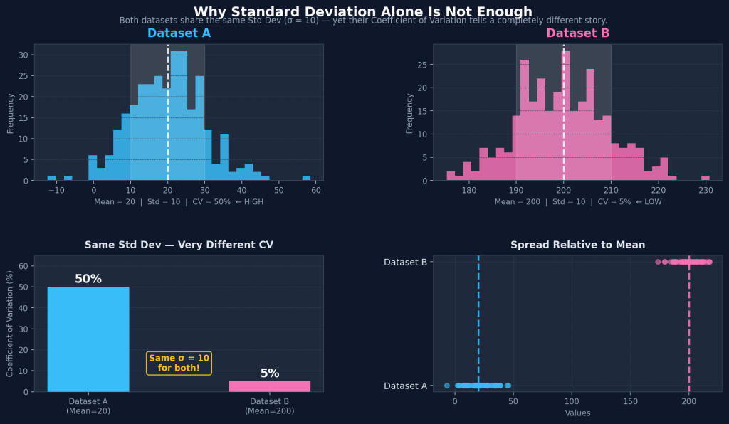
Dataset B (mean=200) has a CV of just 5%. Same standard deviation, completely different story.
This is the question most tutorials skip. Here’s the honest answer:
| Situation | Use Standard Deviation | Use CV |
|---|---|---|
| Comparing spread within one dataset | ✅ | ✅ |
| Comparing two datasets with the same unit | ✅ | ✅ |
| Comparing two datasets with different units | ❌ | ✅ |
| Comparing datasets with very different means | ❌ | ✅ |
| The mean is close to zero | ✅ | ❌ (CV becomes unstable) |
| Data contains negative values | ✅ | ❌ (CV loses meaning) |
The key rule: whenever your question is “which dataset is relatively more spread out?”, reach for the CV. If your question is “how far from the mean is a typical data point, in real units?”, use the standard deviation.
Interpreting CV values: What is a “good” CV?
There’s no universal answer, it depends heavily on your domain. Here’s a practical reference:
| CV Value | Interpretation | Typical Context |
|---|---|---|
| < 10% | Low variability, very consistent data | Lab measurements, manufacturing QC |
| 10% – 30% | Moderate variability | Biological data, social science surveys |
| 30% – 60% | High variability | Financial returns, sales data |
| > 60% | Very high variability | Could signal outliers, heterogeneous data |
A few domain-specific rules of thumb
In manufacturing / quality control: a CV under 10% is typically acceptable. It means your process produces consistent output.
In finance: a higher CV is expected, market returns are inherently volatile. Here, CV is used to compare the risk-per-unit-of-return across different assets.
In machine learning feature analysis: features with very low CV (close to 0%) are nearly constant and carry little predictive value. Features with very high CV may be dominated by outliers.
Coefficient of variation for feature selection in ML
This is where the CV goes beyond textbook statistics and becomes a genuine ML tool.
The core idea
When building a model, you want features that vary enough to be informative. A feature that takes almost the same value for every observation teaches your model nothing. The CV is a fast, unit-free filter to identify these dead-weight features.
This approach is called variance-based filter feature selection, and the CV improves on raw variance by normalizing across scale.
Practical example: Removing low-CV features
python
import pandas as pd
import numpy as np
from sklearn.datasets import load_breast_cancer

# Load dataset
data = load_breast_cancer()
df = pd.DataFrame(data.data, columns=data.feature_names)

# Calculate CV for all features
cv_scores = (df.std() / df.mean()) * 100
cv_df = pd.DataFrame({'Feature': df.columns, 'CV (%)': cv_scores.values})
cv_df = cv_df.sort_values('CV (%)', ascending=True)

print(cv_df.to_string(index=False))
Output (sample):
                    Feature     CV (%)
          mean fractal dimension      6.32
               mean smoothness      7.14
                 mean symmetry      8.56
       mean compactness       48.21
       worst area           86.34
...
Filtering out low-CV features
python
# Set a CV threshold (e.g., remove features with CV < 10%)
threshold = 10
selected_features = cv_df[cv_df['CV (%)'] >= threshold]['Feature'].tolist()

df_filtered = df[selected_features]
print(f"Features kept: {len(selected_features)} out of {len(df.columns)}")
This is a simple, interpretable pre-processing step that runs in milliseconds, no model training required. It works best as a first filter before applying more sophisticated methods like mutual information or LASSO.
Pro tip: combine CV filtering with variance threshold from scikit-learn for a robust, two-step approach that removes both near-zero variance and near-zero relative variance features.
Real-world data science examples
1. Comparing sensor readings across different scales
A smart factory collects temperature (in °C, typical values: 400–600) and vibration frequency (in Hz, typical values: 0.5–3.0). You need to know which sensor is more erratic.
Standard deviation would make temperature look far more variable just because of scale. CV normalizes this and gives you the true comparison.
2. Evaluating model consistency across cross-validation folds
python
import numpy as np

# Accuracy scores across 5 CV folds
model_a_scores = [0.91, 0.89, 0.93, 0.90, 0.92]
model_b_scores = [0.95, 0.81, 0.97, 0.78, 0.93]

def cv_score(scores):
    return (np.std(scores, ddof=1) / np.mean(scores)) * 100

print(f"Model A CV: {cv_score(model_a_scores):.2f}%")
print(f"Model B CV: {cv_score(model_b_scores):.2f}%")
Output:
Model A CV: 1.52%
Model B CV: 8.91%
Model B has a higher average accuracy but is far more inconsistent.
Model A is more reliable in production. The CV makes this visible at a glance.
3. Risk assessment in finance
You’re comparing two investment portfolios. Portfolio A yields 12% average return with an 8% std dev. Portfolio B yields 20% average return with a 18% std dev.
- Portfolio A CV: (8/12) × 100 = 66.7%
- Portfolio B CV: (18/20) × 100 = 90%
CV B offers higher returns but takes on proportionally more risk per unit of return.
🔥 Applying data science to grow a business? If you’re building or scaling an online store, especially in Algeria or globally, check out Ayor.ai. It’s an AI-powered e-commerce platform that uses the kind of data-driven logic we explore in this blog: automation, product optimization, and AI assistants that help you focus on results, not busywork.
CV limitations: When not to use it
The CV is powerful, but it comes with real limitations you need to know before applying it blindly.
- The mean must be non-zero. First and foremost, if your mean is zero or close to zero, the CV approaches infinity and becomes meaningless. For example, CV is useless for data centered around zero (temperature in Celsius, profit/loss ratios).
- CV requires a ratio scale. Beyond that, the data must have a true zero point. You can use CV on height, weight, income, or reaction time. You cannot use it on Celsius temperatures or IQ scores — both are interval scales without a true zero.
- Negative values break the interpretation. Even when the mean is non-zero, if your dataset contains negative numbers and the mean is negative, the CV formula still produces a number, but it loses its intuitive meaning entirely.
- CV is not robust to outliers. Finally, since it’s based on the mean and standard deviation, a single extreme value can distort both and inflate the CV dramatically. In that case, consider using the IQR-based equivalent: Quartile Coefficient of Dispersion (QCD).
python
# QCD: a robust alternative to CV for skewed/outlier-heavy data
def quartile_cv(data):
    q1 = np.percentile(data, 25)
    q3 = np.percentile(data, 75)
    return (q3 - q1) / (q3 + q1)
FAQ
Q: Can the coefficient of variation be greater than 100%? Yes.
A CV above 100% means the standard deviation is larger than the mean, indicating extremely high variability. This is common in right-skewed distributions like income or transaction amounts.
Q: Can CV be negative? Technically, if the mean is negative, the formula produces a negative value.
But this is undefined in the traditional sense, CV is only meaningful when the mean is positive.
Q: What’s the difference between CV and relative standard deviation (RSD)? They are the same thing.
RSD is the term preferred in chemistry and laboratory sciences; CV is more common in statistics and data science.
Q: What is a good CV for machine learning features? There’s no universal cutoff.
A common practice is to drop features with CV below 5–10% as they carry little discriminative signal. But always validate this with domain knowledge, a medical biomarker with 4% CV might still be clinically significant.
Q: How do I calculate CV in pandas for grouped data?
python
df.groupby('category')['value'].agg(lambda x: x.std() / x.mean() * 100)Q: Is CV the same as standard deviation divided by mean? Yes, that’s the exact formula. Multiply by 100 to express it as a percentage.
Conclusion
The Coefficient of Variation is one of the most underused tools in a data scientist’s statistical toolkit. It solves a problem that standard deviation cannot: making variability comparable across different scales and units.
Whether you’re comparing sensor data, evaluating model consistency, screening features before training, or assessing financial risk, CV gives you a normalized, interpretable measure in a single number.
The Python implementations above are ready to plug directly into your EDA or preprocessing pipeline.
Keep building your statistical toolkit
If you found this useful, these guides cover related concepts that every data scientist should have in their toolkit:
- Understanding the Interquartile Range (IQR), The robust alternative to standard deviation for skewed data and outlier detection.
- Prediction Metrics in Machine Learning, Once your features are selected, here’s how to evaluate what your model actually learns.
Together, these three articles give you a complete statistical foundation for clean, reliable data science work.
👉 Join the Around Data Science community on Discord, subscribe to our newsletter, and follow us on LinkedIn for more free resources, tutorials and career tips.



0 Comments