In the world of machine learning, evaluating your model’s predictions is just as important as building the model itself. Prediction metrics, also called forecasting evaluation metrics or model performance metrics, give you a quantitative, objective way to measure accuracy and identify weaknesses before deploying your model.

Whether you are forecasting sales, stock prices, energy demand, or any time series, choosing the wrong metric can lead to wrong conclusions. This complete guide covers 11 essential prediction metrics, explains when to use each one, provides real Python examples, and helps you choose the right metric for your use case.

Quick answer — What is RMSE? RMSE (Root Mean Squared Error) measures the square root of the average squared differences between predicted and actual values. It penalizes large errors heavily. Lower RMSE = better model.

Why Prediction Metrics Are Essential in Machine Learning

Before diving into formulas, let’s understand why choosing the right evaluation metrics for time series forecasting matters so much.

Imagine two models predicting daily electricity demand:

• Model A has 10 small errors of 5 kWh each
• Model B has 1 large error of 50 kWh and 9 perfect predictions

Both models have the same total error (50 kWh), but their risk profiles are completely different. RMSE would flag Model B as worse, while MAE would treat them equally. The right metric depends on your problem.

In time series forecasting specifically, the challenge is even greater because:

• Errors in one period can propagate into future predictions
• Data has seasonality, trends, and autocorrelation
• A “naïve” baseline (predicting yesterday’s value) is often hard to beat
• Scale varies, predicting sales in units vs. revenue in millions needs scale-free metrics

Explore : A/B Testing: A Data-Driven Approach to Boost Fast-Food Sales – Around Data Science

Key Prediction Metrics with Python Examples

1. Root Mean Squared Error (RMSE)

What it measures: Average magnitude of error, with large errors penalized more.

Formula:

Where:

When to use: When large errors are unacceptable (e.g., demand forecasting, medical predictions). RMSE is the most widely used forecasting metric in research and competitions.

Python example:

Imagine you are forecasting daily sales for a store over a week:

Day	Actual Sales \(y_i\)	Predicted Sales ${}_i^{}$ {}^{}{}^{}$$
1	200	210
2	180	170
3	220	215
4	190	200
5	210	205
6	230	240
7	250	245

Using the formula, you can calculate RMSE for this forecast.

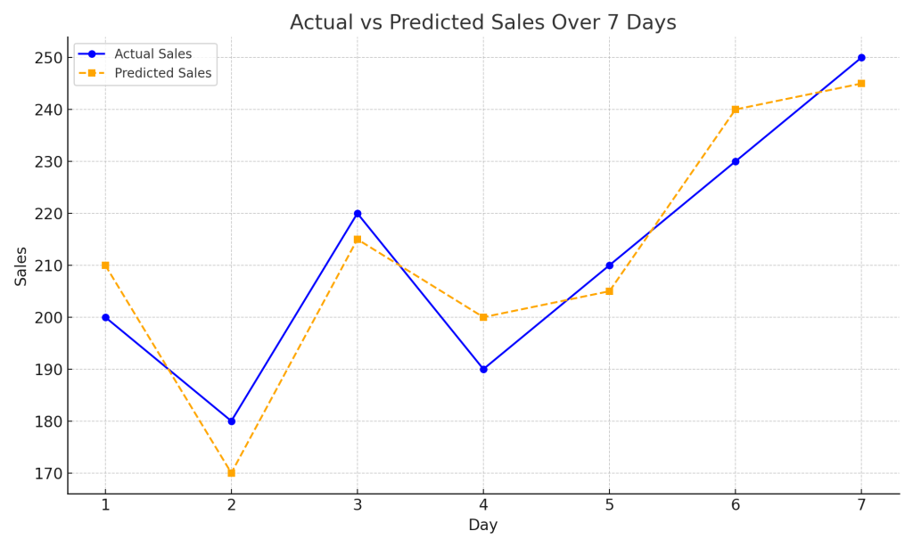
The errors are squared, averaged, and then the square root is taken. A lower RMSE indicates better model performance.

Limitation: Sensitive to outliers. A single large error can dramatically inflate RMSE.

2. Mean Absolute Error (MAE)

What it measures: Average absolute difference between actual and predicted values.

Formula:

When to use: When all errors are equally important, or when you want a metric that is robust to outliers. MAE is easy to explain to non-technical stakeholders.

Python example:

from sklearn.metrics import mean_absolute_error

mae = mean_absolute_error(actual, predicted)
print(f"MAE: {mae:.2f}")
# Output: MAE: 8.57

MAE vs RMSE: If RMSE >> MAE, your model has some very large errors that you should investigate. If they are similar, errors are spread relatively evenly.

3. Mean Absolute Percentage Error (MAPE)

What it measures: Average percentage error, scale-free, easy to interpret.

Formula:

\(MAPE = \frac{1}{n} \sum_{i=1}^{n} \left| \frac{y_i – \hat{y}_i}{y_i} \right| \times 100\)

When to use: When comparing models across datasets with different scales, or when reporting to business stakeholders who think in percentages.

Python example:

def mape(actual, predicted):
    return np.mean(np.abs((actual - predicted) / actual)) * 100

print(f"MAPE: {mape(actual, predicted):.2f}%")
# Output: MAPE: 4.63%

Critical limitation: MAPE breaks when actual values are zero or near zero (division by zero). It is also asymmetric, overestimation and underestimation with the same magnitude produce different MAPE values.

4. Symmetric Mean Absolute Percentage Error (sMAPE)

What it measures: A symmetric version of MAPE that avoids its asymmetry problem.

Formula:

\(sMAPE = \frac{1}{n} \sum_{i=1}^{n} \frac{|y_i – \hat{y}_i|}{\frac{|y_i| + |\hat{y}_i|}{2}} \times 100\)

When to use: When actual values can be small, or when you need symmetric treatment of over- and under-estimation. Widely used in forecasting competitions (M3, M4).

Python example:

def smape(actual, predicted):
    denominator = (np.abs(actual) + np.abs(predicted)) / 2
    return np.mean(np.abs(actual - predicted) / denominator) * 100

print(f"sMAPE: {smape(actual, predicted):.2f}%")
# Output: sMAPE: 4.56%

5. Root Mean Squared Scaled Error (RMSSE)

What it measures: RMSE scaled against a naïve (seasonal random walk) baseline. Values < 1 mean your model beats the naïve forecast.

Formula:

\(RMSSE = \frac{RMSE}{\text{Naïve RMSE}}\)

where Naïve RMSE uses the last observed value as the prediction for the next period.

When to use: Benchmarking your model against a simple baseline. Essential metric in the M5 Forecasting Competition. Useful when comparing models across time series with different scales.

Python example:

def rmsse(actual, predicted, train):
    """
    actual: test set actual values
    predicted: model predictions
    train: training data (for naïve baseline)
    """
    naive_errors = np.diff(train)  # y_t - y_{t-1}
    naive_mse = np.mean(naive_errors**2)
    model_mse = np.mean((actual - predicted)**2)
    return np.sqrt(model_mse / naive_mse)

# RMSSE < 1 → beats naïve forecast

6. Bias (Mean Error)

What it measures: Whether your model systematically overestimates or underestimates.

Formula:

\(Bias = \frac{1}{n} \sum_{i=1}^{n} (\hat{y}_i – y_i)\)

When to use: Always check bias alongside RMSE/MAE. A model with low RMSE but high bias is dangerous — it consistently drifts in one direction.

Python example:

bias = np.mean(predicted - actual)
print(f"Bias: {bias:.2f}")
# Positive bias → model overestimates
# Negative bias → model underestimates
# Output: Bias: 1.43 (slight overestimation)

Interpretation:

• Positive bias: Model predicts higher than reality → risk of over-stocking, over-budgeting
• Negative bias: Model predicts lower than reality → risk of shortages, missed demand

7. Coefficient of Determination (R²)

What it measures: Proportion of variance in actual data explained by the model.

Formula:

\(R^2 = 1 – \frac{\sum (y_i – \hat{y}_i)^2}{\sum (y_i – \bar{y})^2}\)

Where \(\bar{y}\) is the mean of the actual values.

When to use: Primarily in regression tasks. Gives an intuitive 0–1 score (higher is better). Use with caution in time series — R² can be misleadingly high when autocorrelation is present.

Python example:

from sklearn.metrics import r2_score

r2 = r2_score(actual, predicted)
print(f"R²: {r2:.4f}")
# Output: R²: 0.9611

Warning: An R² close to 1 does not always mean a good time series model. Always combine with other metrics.

8. Mean Absolute Scaled Error (MASE)

When to use: The preferred metric for time series forecasting according to Rob Hyndman (author of the forecast R package). Works across different scales and handles zeros.

What it measures: MAE of the model divided by MAE of a naïve in-sample forecast. Scale-free and works even with zero values.

Formula:

\(MASE = \frac{MAE}{\frac{1}{n-1} \sum_{i=2}^{n} |y_i – y_{i-1}|}\)

Python example:

def mase(actual, predicted, train):
    mae_model = np.mean(np.abs(actual - predicted))
    mae_naive = np.mean(np.abs(np.diff(train)))
    return mae_model / mae_naive

# MASE < 1 → your model beats the naïve forecast

9. Directional Accuracy (DA)

What it measures: Percentage of time the model correctly predicts the direction of change (up or down). Critical in finance and demand planning.

Formula:

\(DA = \frac{1}{n-1} \sum_{i=2}^{n} \mathbf{1}\left[\text{sign}(\hat{y}_i – \hat{y}_{i-1}) = \text{sign}(y_i – y_{i-1})\right] \times 100\)

When to use: When the direction of change matters more than the exact value, stock price movement, temperature trends, demand direction.

Python example:

def directional_accuracy(actual, predicted):
    actual_dir    = np.sign(np.diff(actual))
    predicted_dir = np.sign(np.diff(predicted))
    return np.mean(actual_dir == predicted_dir) * 100

da = directional_accuracy(actual, predicted)
print(f"Directional Accuracy: {da:.1f}%")
# Output: Directional Accuracy: 83.3%

10. Congruence (Forecast Stability)

What it measures: How stable and consistent predictions are across the forecast horizon, introduced by Kourentzes. High congruence means your model doesn’t wildly fluctuate between periods.

When to use: Long-horizon forecasting (12+ months), supply chain planning, scenarios where forecast instability has operational costs.

A highly congruent forecast avoids the “nervous forecast” problem where predictions swing from high to low with no clear pattern, making operational planning impossible.

11. Pinball Loss (Quantile Loss)

What it measures: Accuracy of probabilistic forecasts, instead of predicting a single value, you predict a range (e.g., 10th–90th percentile).

Formula:

\(L_\tau(y, \hat{q}\tau) = \begin{cases} \tau \cdot (y – \hat{q}\tau) & \text{if } y \geq \hat{q}\tau \ (1-\tau) \cdot (\hat{q}\tau – y) & \text{otherwise} \end{cases}\)

When to use: Probabilistic forecasting, risk management, when you need prediction intervals rather than point estimates. Used extensively in energy demand forecasting.

Python example:

def pinball_loss(actual, predicted_quantile, tau):
    errors = actual - predicted_quantile
    return np.mean(np.where(errors >= 0, tau * errors, (tau - 1) * errors))

# tau = 0.9 → 90th percentile forecast

Learn more : Top 9 Machine Learning Algorithms Every Beginner Must Know | Around Data Science

Quick Reference: Metrics Comparison Table

Metric	Scale-free	Handles zeros	Penalizes outliers	Best for
RMSE	❌	✅	🔴 Heavy	General ML, competitions
MAE	❌	✅	🟡 Moderate	Robust evaluation
MAPE	✅	❌	🟡 Moderate	Business reporting
sMAPE	✅	⚠️ Partial	🟡 Moderate	Forecasting competitions
MASE	✅	✅	🟡 Moderate	Time series (recommended)
RMSSE	✅	✅	🔴 Heavy	Benchmarking vs. naïve
R²	✅	✅	❌ None	Regression tasks
Bias	❌	✅	❌ None	Systematic error detection
DA	✅	✅	❌ None	Finance, trend prediction
Pinball	✅	✅	🟡 Moderate	Probabilistic forecasting

How to Choose the Right Metric

Use this decision tree to select your evaluation metric(s):

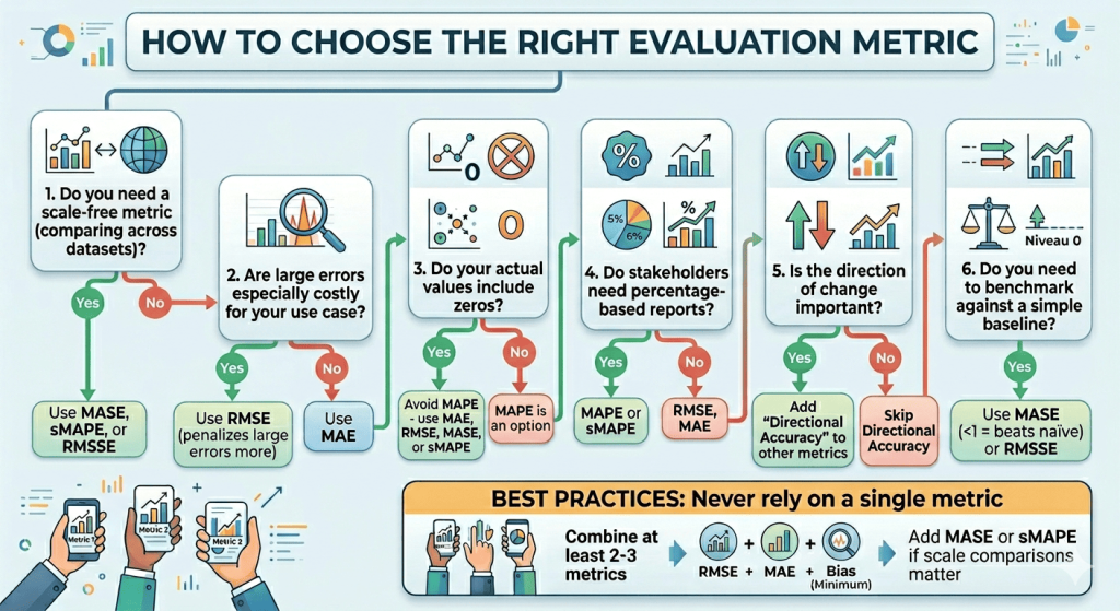
1. Do you need a scale-free metric (comparing across datasets)? → Yes: Use MASE, sMAPE, or RMSSE → No: RMSE or MAE

2. Are large errors especially costly in your use case? → Yes: Use RMSE (penalizes large errors more) → No: Use MAE

3. Do your actual values include zeros? → Yes: Avoid MAPE — use MAE, RMSE, MASE, or sMAPE → No: MAPE is an option

4. Do stakeholders need percentage-based reports? → Yes: MAPE or sMAPE → No: RMSE, MAE

5. Is the direction of change important? → Yes: Add Directional Accuracy alongside other metrics → No: Skip DA

6. Do you need to benchmark against a simple baseline? → Yes: Use MASE (< 1 = beats naïve) or RMSSE

Best practice: Never rely on a single metric. Combine at least 2-3 metrics, typically RMSE + MAE + Bias as a minimum, and add MASE or sMAPE if scale comparisons matter.

Ready to see a proof of concept? Check out this case study : House Prices Prediction using Linear Regression Model – Around Data Science

Practical Example: Evaluating a Sales Forecast with Python

Here is a complete evaluation workflow for a weekly sales forecast:

import numpy as np
from sklearn.metrics import mean_squared_error, mean_absolute_error, r2_score

# Weekly sales data
actual    = np.array([200, 180, 220, 190, 210, 230, 250])
predicted = np.array([210, 170, 215, 200, 205, 240, 245])

# Training data for MASE baseline
train = np.array([160, 175, 185, 195, 200, 190, 205, 198])

# --- Core metrics ---
rmse = np.sqrt(mean_squared_error(actual, predicted))
mae  = mean_absolute_error(actual, predicted)
bias = np.mean(predicted - actual)
r2   = r2_score(actual, predicted)

# --- Scale-free metrics ---
mape_val  = np.mean(np.abs((actual - predicted) / actual)) * 100
smape_val = np.mean(np.abs(actual - predicted) / ((np.abs(actual) + np.abs(predicted)) / 2)) * 100
mase_val  = mae / np.mean(np.abs(np.diff(train)))

# --- Direction ---
da = np.mean(np.sign(np.diff(actual)) == np.sign(np.diff(predicted))) * 100

print("="*40)
print("   MODEL EVALUATION REPORT")
print("="*40)
print(f"RMSE:  {rmse:.2f}")
print(f"MAE:   {mae:.2f}")
print(f"Bias:  {bias:.2f}  ({'overestimates' if bias > 0 else 'underestimates'})")
print(f"R²:    {r2:.4f}")
print(f"MAPE:  {mape_val:.2f}%")
print(f"sMAPE: {smape_val:.2f}%")
print(f"MASE:  {mase_val:.3f}  ({'beats' if mase_val < 1 else 'does NOT beat'} naïve)")
print(f"DA:    {da:.1f}%")

Output:

========================================
   MODEL EVALUATION REPORT
========================================
RMSE:  10.35
MAE:   8.57
Bias:  1.43  (overestimates)
R²:    0.9611
MAPE:  4.63%
sMAPE: 4.56%
MASE:  0.571  (beats naïve)
DA:    83.3%

Reading these results:

The model is performing well overall (MAPE ~4.6%, MASE < 1 means it beats the naïve baseline), but has a slight tendency to overestimate (positive bias = +1.43 units/day). The 83.3% directional accuracy means it correctly predicts whether sales go up or down in 5 out of 6 transitions.

Frequently Asked Questions

What is the difference between RMSE and MAE?

Both measure average prediction error, but RMSE squares the errors before averaging, making it more sensitive to large errors. If you have occasional large errors that you want to penalize heavily, use RMSE. For robust evaluation where all errors matter equally, use MAE.

What does RMSE mean in practice?

RMSE has the same unit as your target variable. An RMSE of 10 when forecasting daily sales means your model is off by about 10 units on average (with larger errors weighted more). Compare it to the scale of your data: an RMSE of 10 on sales of 200 units (~5%) is excellent; on sales of 15 units (~67%) it is poor.

What is a good MAPE value?

As a rule of thumb: MAPE < 10% is excellent, 10–20% is good, 20–50% is acceptable, > 50% is poor. However, this depends heavily on the domain, financial forecasting tolerates higher MAPE than, say, inventory management.

Why is MASE recommended for time series?

MASE (Mean Absolute Scaled Error) is scale-free and handles zero values, making it ideal for comparing models across different time series. A MASE < 1 means your model outperforms a naïve “predict yesterday’s value” forecast, giving an automatic benchmark.

Should I use R² for time series forecasting?

Use R² with caution for time series. Because time series data is autocorrelated, R² can appear high even for poor models. It works better for cross-sectional regression. Prefer MASE, RMSSE, or MAPE for time series evaluation.

What metric does the M5 Forecasting Competition use?

The M5 Competition (the most prestigious forecasting benchmark) uses RMSSE (Root Mean Squared Scaled Error). Understanding this metric is essential if you follow forecasting research.

Conclusion

Prediction metrics are the foundation of honest model evaluation. The key takeaways from this guide:

• RMSE for general ML — penalizes large errors, widely understood
• MAE for robust evaluation — not skewed by outliers
• MAPE / sMAPE for business reporting — percentage-based, intuitive
• MASE / RMSSE for time series — scale-free, benchmarks against naïve
• Bias to detect systematic drift — always check alongside other metrics
• Directional Accuracy when trend direction matters more than magnitude
• Pinball Loss for probabilistic forecasting

Always use at least 2-3 metrics together, no single metric tells the complete story. And always check your Bias separately, as a model can have low RMSE while systematically drifting in one direction.

🌟For more in-depth guides and resources, explore Around Data Science hub. Dive deeper into specific topics, discover cutting-edge applications, and stay updated on the latest advancements in the field. Subscribe to our newsletter to receive regular updates and be among the first to know about exciting new resources, like our first free eBook on Artificial Intelligence for All! Don’t miss out!

Welcome to a world where data reigns supreme, and together, we’ll unravel its intricate paths